QM/EFP calculations using BioEFP and FlexEFP

Introduction

QM/EFP methods are powerful tools for describing photo- and redox-chemistry in condensed phases, see e.g., Biological chromophores. However, setting up QM/EFP calculations for complex systems is not trivial and time-consuming. This tutorial presents a computational workflow that helps interested users to set up QM/EFP calculations of photoactive proteins in a format suitable for calculations in Q-Chem. It is assumed that the initial structures for QM/EFP calculations are obtained from a GROMACS MD trajectory. GAMESS is used for computing EFP parameters.

The workflow was tested on several photosynthetic pigment-protein complexes (FMO, PS1, WSCP). While the workflow is reasonably general and can be adapted to other biological and materials systems, the QM/EFP calculations are not black-box procedures and the user will need to make decisions based on the system specifics and the properties of interest.

The following scripts are covered in this tutorial:

make_AAs.py — prepares GAMESS MAKEFP input files for all EFP region fragments
cut_caps.py — trims EFP parameter files by removing capping hydrogens and correcting charges
make_qchem_input.py — assembles the final Q-Chem QM/EFP input file

Preliminaries

The following software is required:

GROMACS
GAMESS
Q-Chem
libEFP
Python 3 (with numpy)

To start with, you will need the following GROMACS files:

structure file (.g96)
topology file (.top)
binary run input file (.tpr)

If you wish to use the FlexEFP scheme as described in Flexible EFP paper, you also need a library of precomputed EFP potentials. The parameter database from the Flexible EFP paper can be found here.

Workflow overview

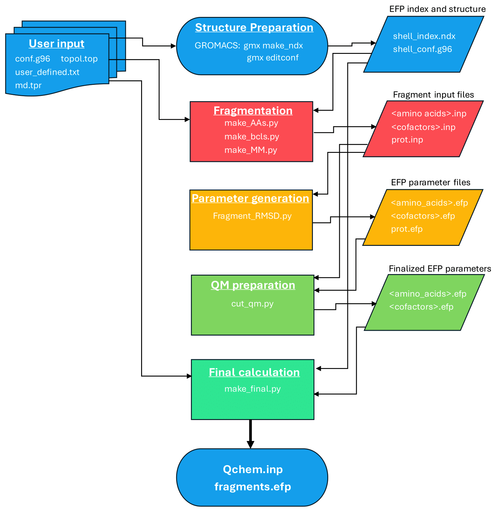
The workflow leads the user through the following steps:

Defining QM and EFP regions
Fragmentation of the EFP region
EFP parameter generation
EFP parameter trimming
QM/EFP input generation

FMO protein

The Fenna-Matthews-Olson (FMO) protein is used as an example system throughout this tutorial. Preparation of the QM and EFP regions follows the work by Kim et al..

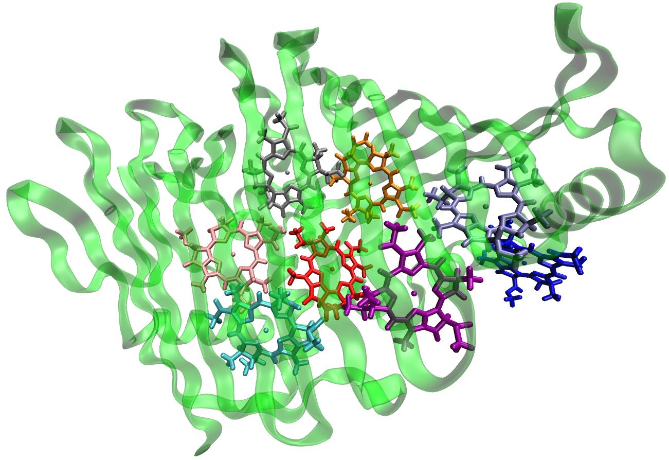
FMO is a trimeric protein with eight bacteriochlorophyll a (BChl) pigments in each monomer. FMO facilitates energy transfer via excitonic couplings across these eight BChls.

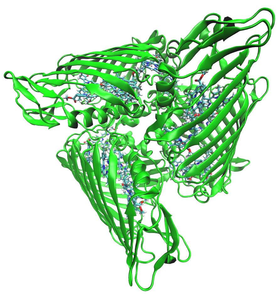
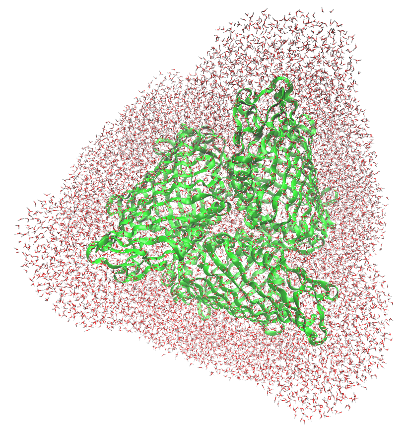
In the present example, water molecules more than 15 Angstroms from the protein surface have been removed.

Molecular dynamics and constrained QM/MM geometry optimizations have been performed on the system prior to this tutorial. Constrained QM/MM geometry optimizations have been shown to be essential for accurate predictions of optical spectra and redox properties. However, this step is not covered here and it is left to the user to perform if needed.

Note

The provided .g96 file contains QSL and LA residues, corresponding to “quantum” waters (water molecules included in the QM region during QM/MM optimizations) and link atoms that were utilized in QM/MM optimizations, respectively. These are left over from the QM/MM optimization step and are not required for any of the scripts in this tutorial.

Defining QM and EFP regions

In the present example, the QM/EFP calculation will be set up for the third BChl (residue number 361) in the active (QM) region.

EFP region

While it is possible to include all non-QM atoms in the EFP region, this approach can be computationally expensive for larger proteins for computing EFP parameters and performing QM/EFP calculations. A practical approach is to define an EFP region that includes all residues within a particular distance from the QM region. Here, we include every amino acid, non-QM BChl, and water molecule containing at least one atom within 15 Angstroms of the BChl chlorin ring.

Note

A single snapshot can be extracted from a GROMACS MD trajectory in .g96 format using:

gmx trjconv -s md_50.tpr -f md_50.trr -o snapshot_50000.g96 -dump 50000

Note

Extracting larger systems can occasionally cause columns to be misaligned when the: residue ID passes from 9999 to 10000. This misalignment can make the structure appear incorrectly in VMD or other visualizers (e.g., “sheets” of waters with misread coordinates). Though it shouldn’t matter for this tutorial, you can fix the problem by realigning the columns.

Column reformatting script is an example of a script that can fix this problem.

To determine which residues constitute the EFP region, we use the gmx select command. First, create an index file defining the BChl headring group containing the atoms of the chlorin ring:

Note

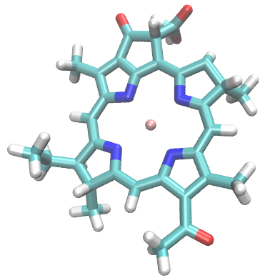
The BChl chlorin ring (headring) is defined by the following atom names: MG CHA CHB HB CHC HC CHD HD NA C1A C2A H2A C3A H3A C4A CMA HMA1 HMA2 HMA3 NB C1B C2B C3B C4B CMB HMB1 HMB2 HMB3 CAB OBB CBB HBB1 HBB2 HBB3 NC C1C C2C H2C C3C H3C C4C CMC HMC1 HMC2 HMC3 CAC HAC1 HAC2 CBC HBC1 HBC2 HBC3 ND C1D C2D C3D C4D CMD HMD1 HMD2 HMD3 CAD OBD CBD HBD CGD O1D O2D CED HED1 HED2 HED3

The following code generates the index file (index.ndx) containing all standard GROMACS index groups with the new headring group appended:

gmx make_ndx -f formed_bchl361-79002.g96 <<EOF
r 361 & a MG CHA CHB HB CHC HC CHD HD NA C1A C2A H2A C3A H3A C4A CMA HMA1 HMA2 HMA3 NB C1B C2B C3B C4B CMB HMB1 HMB2 HMB3 CAB OBB CBB HBB1 HBB2 HBB3 NC C1C C2C H2C C3C H3C C4C CMC HMC1 HMC2 HMC3 CAC HAC1 HAC2 CBC HBC1 HBC2 HBC3 ND C1D C2D C3D C4D CMD HMD1 HMD2 HMD3 CAD OBD CBD HBD CGD O1D O2D CED HED1 HED2 HED3
name 26 Headring
q
EOF

Warning

Make sure to adjust the code above to your system’s active region!

Here is a visualization of the atoms contained in the newly created index group:

The following command selects all residues containing at least one atom within 1.5 nm (15 Angstroms) of the headring group and writes them to a new index file:

gmx select -s md_80.tpr -n index.ndx -f bchl361-79002.g96 -select 'same residue as within 1.5 of group "Headring"' -on shell_index.ndx

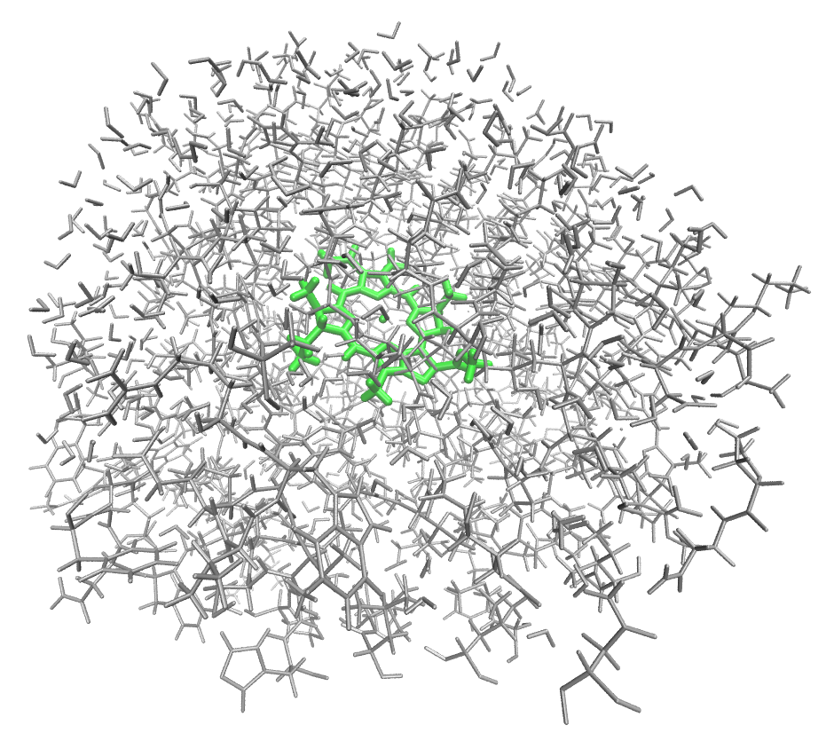
The output shell_index.ndx contains exactly one index group defining the EFP region. Next, extract the EFP region into a new structure file:

gmx editconf -f formed_bchl361-79002.g96 -n shell_index.ndx -o shell_bchl361-79002.g96

Note that no output group needs to be specified since shell_index.ndx contains only one group. The resulting EFP shell surrounding the headring looks like this:

Note

The QM region will include the entire BChl, but the EFP region is defined by distance to the chlorin ring only.

QM region

Warning

Defining the QM region is system-specific. The user must prepare a text file containing all atoms of the QM region as well as pairs of atoms defining any covalent boundaries between the QM and EFP regions.

An example file prepared for the third BChl in FMO is provided: qm_defined.txt. This file can be constructed by copying the corresponding lines from the .g96 file. The QM_atoms section should contain all QM atoms, not including capping hydrogens for covalent QM-EFP boundaries.

QM_atoms
HID   CB      4423    7.642829418    5.747635365    6.631662846
HID   HB1     4424    7.690435886    5.791911602    6.719151974
HID   HB2     4425    7.702376842    5.734309196    6.541343212
HID   CG      4426    7.616473675    5.602392197    6.675217152
HID   ND1     4427    7.564018726    5.549627781    6.790104389
HID   HD1     4428    7.526696682    5.608877659    6.862887859
HID   CE1     4429    7.573244572    5.417556286    6.787623882
HID   HE1     4430    7.525365353    5.356580257    6.862813473
HID   NE2     4431    7.630198002    5.375784874    6.671539783
HID   CD2     4432    7.659914494    5.495519638    6.606870174
HID   HD2     4433    7.729931355    5.498696804    6.524702549
BCL   MG      5807    7.683570385    5.063692570    6.584101200
BCL   CHA     5808    7.531836033    5.139747143    6.278742790
BCL   CHB     5809    7.987795353    5.096710682    6.448209286
BCL   HB      5810    8.083442688    5.096199036    6.395521641
BCL   CHC     5811    7.814235210    5.021772861    6.903957844
BCL   HC      5812    7.851527691    5.018221855    7.006530285
BCL   CHD     5813    7.359744549    5.040185928    6.723926067
BCL   HD      5814    7.258452892    5.027849674    6.762816906
...

The “QM-MM” boundary section is optional and should contain pairs of atoms for each covalent boundary, with the QM atom listed first. The example

qm_defined.txt contains only one QM-MM boundary, but a second boundary could be included like this:

QM-MM
boundary 1
  290 HID   CB      4423    7.642829418    5.747635365    6.631662846
  290 HID   CA      4421    7.514162540    5.827141285    6.594927311
boundary 2
  290 HID   CB      4423    7.642829418    5.747635365    6.631662846
  290 HID   HB1     4424    7.690435886    5.791911602    6.719151974

Note that the atom indexes MUST match those in the structure file, but the coordinates do NOT need to match. If you are planning to run multiple EFP calculations on identically-built structures (e.g. different times of a single MD trajectory), then you can reuse the same QM-defining text file.

Example: QM region for the third BChl in FMO

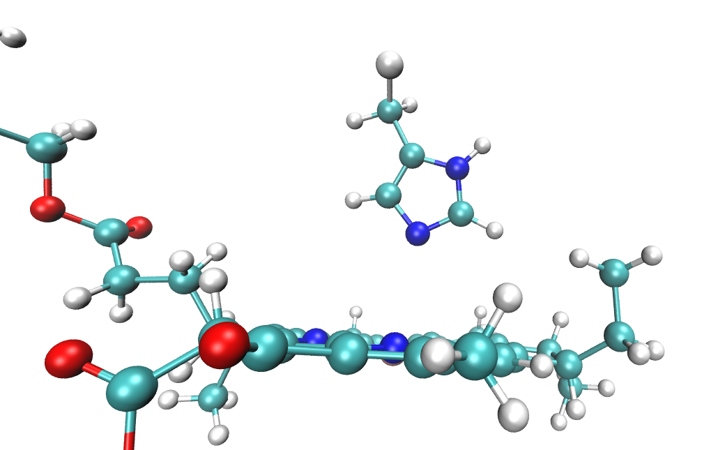
By trial and error we found that including the Mg-coordinating amino acid residue in the QM region in QM/EFP calculations helps SCF convergence and makes excitation energies more reliable. Thus, the QM region will include all atoms of the BChl (residue BCL 361) as well as atoms from the nearby histidine that coordinates the BChl Mg atom shown below.

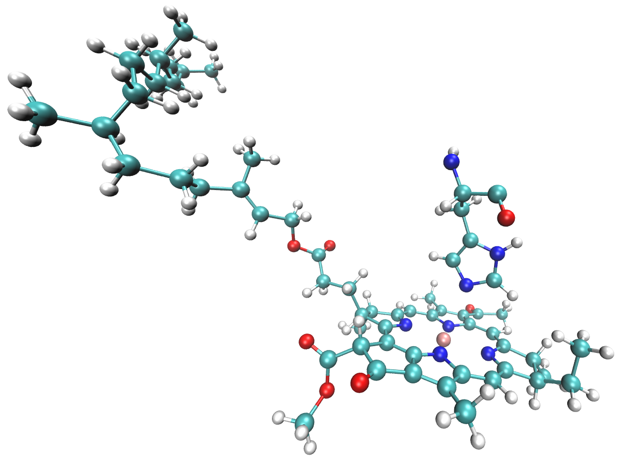
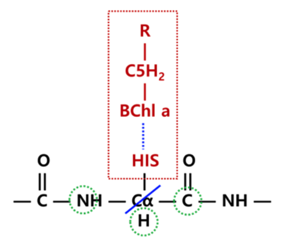
The full residues 361 (BCL) and 290 (HIS) are shown above; however, only the side chain of the histidine is included in the QM region. Specifically, residue atoms from $C_{\beta}$ onward are included, while backbone atoms from $C_{\alpha}$ onward remain in the EFP region:

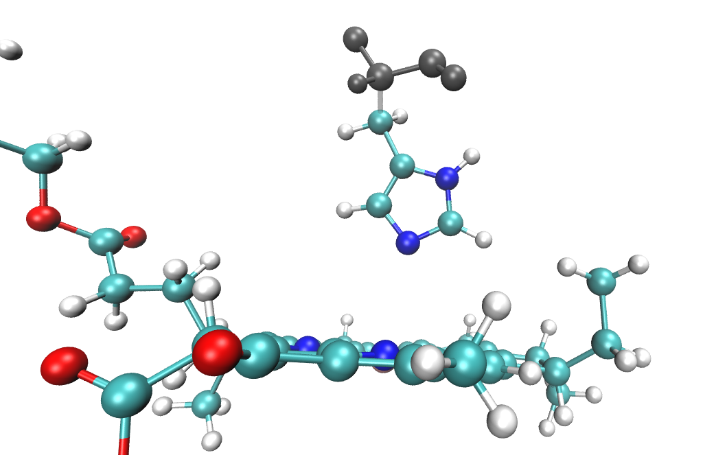
A covalent QM-EFP boundary is therefore defined between $C_{\beta}$ and $C_{\alpha}$. The scripts automatically cap the QM region with hydrogen atoms positioned along the boundary bond, so the QM region in the QM/EFP calculation looks like this:

Preparation of the EFP fragment for the boundary histidine is discussed in QM-EFP boundary fragments.

Fragmentation of the EFP region

Now we need to prepare EFP fragments for our system. In EFP region we have already created a .g96 file containing atoms belonging to the EFP region. Here we will split polypeptide chains and other large residues into EFP fragments.

Splitting protein into EFP fragments

Because proteins tend to be continuous chains, covalent bonds between neighboring amino acids have to be broken for fragmentation. Chemically, the $C-C_{\alpha}$ bond (between alpha carbon and carbonyl carbon) is broken, however, standard PDB convention divides residues by the C-N bond (alpha carbon-nitrogen).

Visually, PDB residues are divided like this:

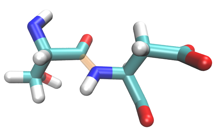
but EFP fragments should be divided like this:

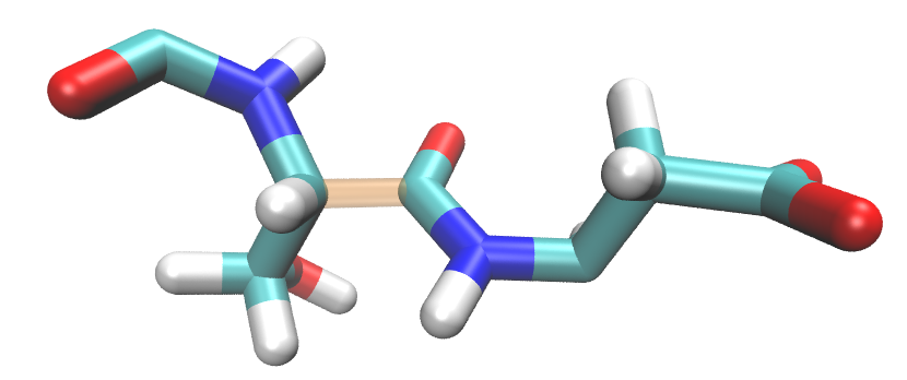
Therefore, EFP amino acid fragments will not completely agree with PDB amino acid numbering. Below is a snippet from the structure file (.g96) with EFP fragment 7 highlighted. Note that atoms C and O of PDB residue 6 (SER) are included in EFP fragment 7 (ASP).

SER   N         75    8.321870804    4.485276699    7.284091473
SER   H         76    8.350618362    4.454034328    7.375734806
SER   CA        77    8.417644501    4.567386150    7.205451488
SER   HA        78    8.419803619    4.528203011    7.103761196
SER   CB        79    8.368366241    4.711947441    7.193405628
SER   HB1       80    8.269208908    4.708506584    7.148269176
SER   HB2       81    8.421850204    4.761358261    7.112295628
SER   OG        82    8.367326736    4.794726372    7.312560558
SER   HG        83    8.454633713    4.832594395    7.325180531
SER   C         84    8.560445786    4.558277130    7.268922329
SER   O         85    8.572677612    4.533203125    7.387583256
ASP   N         86    8.663642883    4.582690239    7.183378696
ASP   H         87    8.638984680    4.619784832    7.092730999
ASP   CA        88    8.804636002    4.563919544    7.209733486
ASP   HA        89    8.821094513    4.593161583    7.313438892
ASP   CB        90    8.842021942    4.416758537    7.207666874
ASP   HB1       91    8.802436829    4.372995377    7.116020679
ASP   HB2       92    8.804891586    4.358578205    7.292031765
ASP   CG        93    8.994537354    4.388171196    7.197051525
ASP   OD1       94    9.062387466    4.408482552    7.298908710
ASP   OD2       95    9.046514511    4.348608971    7.086165905
ASP   C         96    8.905342102    4.655499458    7.132633686
ASP   O         97    8.919197083    4.634913445    7.010179996

A daunting task of splitting the protein into EFP fragments is accomplished by script make_AAs.py. A sample execution is:

python make_AAs.py shell_bchl361-79002.g96 bchl361-79002.g96 qm_defined.txt topol.top <timestep> <mutant>

.g96 file containing atoms of the EFP region (see EFP region)
.g96 file containing the full system (initial structure from MD)
user-prepared file defining the QM region and QM-EFP boundaries (see Defining QM and EFP regions)
topology file (topol.top)
timestamp to differentiate output files (e.g. 50000)
mutant label (e.g. wt)

Output:

GAMESS MAKEFP input files for all amino acid and other residues in the EFP region

Note

GAMESS MAKEFP input file parameters (basis set, memory, etc.) can be adjusted directly in make_AAs.py.

The script splits the EFP region into fragments and creates a GAMESS MAKEFP input file for each. Output filenames are derived from the full system .g96 file. For example, v_22_301_50000_wt.inp corresponds to a valine residue (v), residue number 22, with first atom ID 301 (of the full structure, NOT the structure of the EFP region). Histidine residues are denoted hd_, he_, or hp_ depending on protonation state. Capping hydrogens are added automatically to amino acid fragments, they will always have the atom name H000 (multiple virtual hydrogens will have the same atom name). These will be removed from the EFP parameter files in a later step (see EFP parameter trimming).

Non-standard residues and cofactors are named using the full residue name from the .g96 file (e.g., bcl_360_5667_50000_wt.inp for BCL with residue number 360). Non-amino acid fragments are created without capping hydrogens by default.

QM-EFP boundary fragments

For a fragment with a covalent QM-EFP boundary (e.g., HIS 290 from Example: QM region for the third BChl in FMO), make_AAs.py will append two comment lines to the end of the input file. The !erased: line lists atom names of QM atoms to be removed from the parameter file. The !remove: line additionally lists atoms around which polarization points will be removed, identified by analysis of the topology file. Here is an example for HIS 290 (hd_290_4417_50000_wt.inp):

Note that while $C_{\alpha}$ is not part of the QM region, it is a QM-EFP boundary atom and will also be removed from the parameter file in a later step. These comment lines are used by cut_caps.py to finalize the fragment parameter files (see EFP parameter trimming). The boundary scheme follows the approach developed by Kim et al., which ensures stability of QM/EFP calculations in the FMO protein.

Warning

The QM-EFP boundary scheme for amino acid fragments is general. However, the user may need to modify it for non-standard fragments.

If a residue contains only QM atoms, such as BCL 361 in our example, no input file will be created.

Non-amino acids and cofactors

make_AAs.py handles EFP fragment preparation for standard amino acid sequences, non-covalently linked molecules (e.g., water molecules, ions), and cofactors including (B)Chls. For large cofactors exceeding roughly 100 atoms, the script creates one fragment for the entire residue by default. Sometimes, it is desirable to split a large cofactor into sub-fragments. See below, the separate chlorin head and phytol tail fragments for a BCL.

Below is an example of the head/tail division used for BChl:

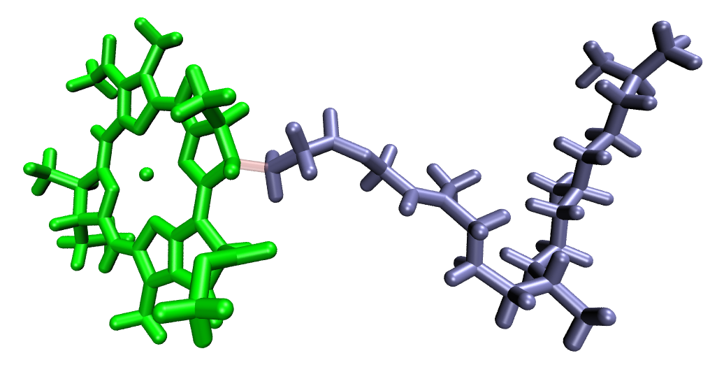
For the BChl case, capping hydrogens are added at the head-tail junction in the same way as for amino acid backbone cuts. CLA, BCL, LMG, and LHG fragments are cut using this script, but note that atom names must match those used in this example setup. The same syntax used for those can be used to create a custom sub-fragmentation scheme. The relevant variables to adjust are contained the define_ligand_cut function, and they are:

RESNAME — residue name to be fragmented
Rings — list of atom names to include in the head fragment; all others go to the tail
headside / tailside — atom names on either side of the covalent cut
site — optional; residue ID of a QM BChl that should be skipped entirely

EFP parameter generation

make_AAs.py from the previous step created a collection of GAMESS MAKEFP input files. You now have two options for obtaining EFP parameters:

Compute all needed EFP parameters by running the MAKEFP inputs in GAMESS
Use the FlexEFP procedure to obtain parameters by rotation of precomputed parameters stored in a database

If your system is small or you do not wish to use the FlexEFP scheme, submit GAMESS calculations for all generated inputs, collect all produced .efp files, and proceed to EFP parameter trimming.

Otherwise, frag_RMSD_V2.py checks the geometry of each fragment against fragments available in the precomputed parameter database. For amino acids, the script searches only among fragments of the same amino acid type. If the RMSD between the two structures is below the threshold, the database parameters are considered transferable and will be rotated and translated to match the geometry of your fragment— no GAMESS calculation needed for that fragment. Note that if the RMSD is greater than the cutoff threshold, you will need to generate the parameters of that fragment in GAMESS. You can add computed parameters to your fragment library to reduce the computation time of future timesteps.

Note

The path to the EFP parameter database is hardcoded in frag_RMSD_V2.py. Adjust it to point to your local copy of the database before running.

Note

The RMSD threshold is hardcoded in frag_RMSD_V2.py to 0.2 Angstroms. Adjust if desired.

The script is run on one single GAMESS MAKEFP input file at a time:

frag_RMSD_V2.py a_4_45_50000_wt.inp

This reads a_4_45_50000_wt.inp (an alanine fragment, identified by the a_ prefix) and computes the RMSD against each .efp file found in the ala/ subdirectory of the database. The database subdirectory is determined automatically from the one-letter amino acid prefix in the filename (e.g., a → ala/, v → val/, etc.).

If no suitable match is found, the script prints:

No match, run GAMESS for: <filename>

and no .efp file is created for that fragment. If no database folder is found, or if the input is not a standard non-terminal amino acid, the script will return an error. All such fragments will need to be computed in GAMESS. Fortunately, most of these calculations will not take more than a few minutes.

A simple way to run frag_RMSD_V2.py on all fragments at once is to iterate over every *.inp file in the current directory using a bash script:

for f in *.inp; do
    python frag_RMSD_V2.py $f
done

After running, any fragment for which no .efp file was produced will need to be submitted to GAMESS. A convenient way to identify these is:

for f in *.inp; do
    base="${f%.inp}"
    if [ ! -f "${base}.efp" ]; then
        echo "No EFP found, submit to GAMESS: $f"
    fi
done

The Classical Region Fragment

Atoms not included in either the QM or EFP regions — i.e., atoms far from the QM subsystem — are treated as classical atoms possessing only partial charges. These are combined into a single EFP “superfragment” containing only coordinates, monopoles, and screen sections.

make_AAs.py will create this, and it should not require any more preparation other than the structure files already provided.

The topology file provides atomic charges. Both structure files are required so that only classical atoms are included — QM and EFP atoms are automatically omitted.

EFP parameter trimming

Before using the EFP parameters in QM/EFP calculations, the fragment parameter files must be trimmed. Specifically:

Capping hydrogens added to amino acid fragments to make them closed-shell molecules for parameter calculations must be removed, along with all associated parameters.
Fragments with covalent QM-EFP boundaries must be cleaned of all QM atoms and boundary atoms. Additionally, polarization points near the boundary must be removed to avoid overpolarization of the QM region.
Sub-fragmented molecules are treated in the same way as amino acid fragments — capping hydrogens at the head-tail junction are removed automatically.

This trimming is handled by cut_caps.py. The script uses the comment lines appended by make_AAs.py (see QM-EFP boundary fragments) to determine which atoms and polarization points to remove.

Note

cut_caps.py will always remove hydrogens named H000 (capping hydrogens added to cap dangling bonds when fragments were cut from a larger molecule) and all associated parameters, regardless of the comment lines in the input file.

QM-EFP boundary fragments are treated based on the !erased: and !remove: comment lines in the input file, as described in QM-EFP boundary fragments.

cut_caps.py operates in two modes: check (default) and fix.

In check mode, the script validates the EFP parameter file for completeness and sanity without modifying it:

Exits with an error if the .efp file is incomplete (missing $end statement)
Exits with an error if the fragment charge is non-integer or if partial charges exceed the charge_cutoff threshold
Prints a warning if large polarizability values are found

In fix mode, the script performs the trimming and writes the result to cut_<efp_filename>.

Note

Check and adjust the charge_cutoff and polab_cutoff settings at the top of cut_caps.py if needed for your system.

A sample execution in check mode:

python cut_caps.py hd_290_4417_50000_wt.inp hd_290_4417_50000_wt.efp

A sample execution in fix mode:

python cut_caps.py hd_290_4417_50000_wt.inp hd_290_4417_50000_wt.efp fix

The two arguments are:

GAMESS MAKEFP input file (.inp) — provides the atom removal instructions via comment lines
EFP parameter file (.efp) — either the direct output of the GAMESS MAKEFP calculation, or a parameter file rotated and translated by frag_RMSD_V2.py

cut_caps.py must be executed for every fragment in the EFP region. A convenient way to run it on all fragments at once is:

for f in *.inp; do
    base="${f%.inp}"
    if [ -f "${base}.efp" ]; then
        python cut_caps.py $f ${base}.efp fix
    fi
done

After trimming, the resulting cut_*.efp files are ready for use in the QM/EFP input generation step.

QM/EFP input generation

Now that all fragment .efp files are prepared, the QM/EFP input file in Q-Chem format can be assembled. This is handled by make_qchem_input.py. A sample execution is:

python make_qchem_input.py shell_bchl361-79002.g96 bchl361-79002.g96 qm_defined.txt topol.top timestamp mutant

The input arguments are very similar to those in make_AAs.py:

.g96 file containing atoms of the EFP region (see EFP region)
.g96 file containing the full system (initial structure from MD)
user-prepared file defining the QM region and QM-EFP boundaries (see Defining QM and EFP regions)
topology file (topol.top)
timestamp to differentiate output files (e.g. 50000)
mutant label (e.g. wt)

The Q-Chem calculation keywords are defined in the build_header function inside make_qchem_input.py and can be adjusted as needed for your calculation type (e.g., excitation energy, redox potential).

Note

When submitting the Q-Chem calculation, all cut_*.efp parameter files must be present in the same directory as the input file, and they MUST be renamed to match the names listed in efp_region.txt (by default, this is the same name without the cut_ prefix). It is convenient to move the cut_*efp files to a new folder to avoid overwriting the original GAMESS outputs.

Note

make_qchem_input.py currently generates input files for Q-Chem only. Users wishing to run QM/EFP calculations in GAMESS will need to adapt the build_header function accordingly.

Time-Saving Tips

In the case of FMO, the typical procedure is to repeat the QM/EFP calculation setup for each of the eight BChl pigments in the monomer. EFP fragments can be reused between calculations if they come from the same MD snapshot. For example, setting up a calculation centered on BChl 360 will require only a small number of new fragments compared to those already generated for BChl 361, since the majority of the EFP shell overlaps. This can save considerable time when setting up repeated calculations across multiple pigments.

A second time-saving strategy is to build and maintain your own library of precomputed EFP fragments for use with the FlexEFP step. In practice, a library built for one protein will often transfer well to structures of the same trajectory, reducing the number of GAMESS calculations needed.

For large-scale studies involving many snapshots, consider wrapping the full pipeline — from make_AAs.py through cut_caps.py to make_qchem_input.py — in a bash or Python driver script that iterates over many snapshots. Note that the primary bottleneck will be waiting for GAMESS to generate fragment parameters.